Face Morphing using Delaunay Triangulation
- Devendra Pratap Yadav
We can use various algorithms to generate the intermediary images while morphing an image say M to another image say N. The parameter α controls the morphing of M to N. The value of α lies between 0 and 1 (inclusive).
α = 0 indicates the original image M (no morphing), whereas α = 1 indicates complete transformation of M to N.
It is assumed that both the images M and N are of the same dimensions.
Naïve Algorithm
We first describe a simple algorithm for morphing between 2 images. This algorithm takes a weighted mean of the pixel intensity values of the original image and the target image, depending on the α parameter. More formally,
I (x, y) = (1 - α) M (x, y) + α N (x, y)
Where I = Intermediate image
M = Original image
N = Target image
This algorithm, however, gives terrible results, if the primary features of the two images (say eyes, nose or other facial features, when morphing between two human portraits) are misaligned. We need to find a one – to – one correspondence between certain parts of the two images, so as to know which part of the original image should be morphed into which part of the target image. This is done by the algorithm described next.
Point to point correspondence and triangulation
The 3 step algorithm is described below:
Step 1: Marking points
In this step, we mark the primary features of both image M and N, establishing a one – to – one correspondence between the points marked in M and N. Let us consider morphing between two human portraits. In this case we would be marking the prominent facial features in both the images, say eyes, eyebrows, nose, lips, chin edge etc. We can use multiple points to adequately cover the major facial features. Also, since this is a one – to – one correspondence, the number of points marked in M will be equal to the number of points marked in N. We can manually mark these points in both the images, or use a software tool to automatically detect these features and mark the points for us.
Step 2: Delaunay Triangulation
After obtaining all the marked points in both the images, we calculate a weighted mean of the points in the two sets, based on the value of α.
Let us suppose the two set of points are:
SM = {m1, m2, m3, ….., mk} and SN = {n1, n2, n3, ….., nk}
We obtain another set of point SI = {i1, i2, i3, ….., ik}, where,
ik = (1 - α) mk + α nk
These are the points for the intermediate image, corresponding to the primary features of the images.
All the three sets of points, namely SM, SI, SN, are stored in three separate text files, separated by newlines. Each text file contains same number of lines (same number of points in SM, SI, and SN), to indicate the one – to – one correspondence.
The next step is to apply the Delaunay Triangulation to the set SI.
Applying Delaunay Triangulation:
Consider the set of points SI as obtained by the above steps. Triangulation operation divides the plane of the image into many small triangles, using the points of the set SI as vertices.
Delaunay Triangulation is one such operation. The triangles chosen by this algorithm are such that no point of the set SI lies inside the circumcircle of any triangle. The advantage of such a property is that it will reject very thin triangles with one very large obtuse angle and two very small angles. Such thin triangles when morphed will not be very perceptible.
The triangulation is performed for all the sets SM, SI, SN, giving a one – to – one correspondence between triangles in the image M, I and N.
There are many algorithms and libraries to calculate the Delaunay Triangulation, given a set of points. We will be using an inbuilt function named Subdiv2D, of OpenCV, which does the triangulation and returns the set of co-ordinates of the triangles thus obtained. This function generates a new text file for each image, containing the indexes of the points used as vertices in the original text files. This is analogous to a Hash Map of the marked points.
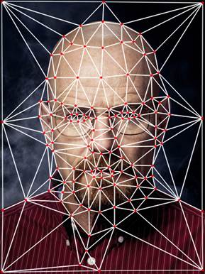
For out set of tie points we obtain the triangulation shown above
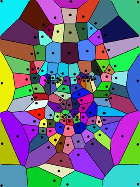
Corresponding Voronoi Diagram for above image.
Step 3: Affine Transformation
We now select a triangle T from the image M, its corresponding triangle V in the intermediate image I, and calculate the affine transform (described below) that converts the triangle T to V. We use the inbuilt function getAffineTransform, in OpenCV, to obtain the transformation matrix. Similarly, we calculate the transformation matrix of the corresponding triangle W in the image N to the triangle V. Now we apply the transformations so obtained to all the triangles of both the images M and N, to obtain warped images M’ and N’ . We next calculate the intermediate image I by using the same equation as the naïve algorithm:
I (x, y) = (1 - α) M’ (x, y) + α N’ (x, y)
We obtain a series of intermediate images based on different values of α, ranging between 0 and 1. These images when shown in rapid succession gives the effect of one image being morphed into the other. More the number of intermediate images, smoother is the transformation from one image to the other.
We have referred to the following sources to aid us in developing the code.
2) https://www.learnopencv.com/delaunay-triangulation-and-voronoi-diagram-using-opencv-c-python/
3) https://www.cs.princeton.edu/courses/archive/fall00/cs426/papers/beier92.pdf
4) http://www.cs.cmu.edu/~quake/triangle.html
Affine transformation between two triangles
Let us suppose we are trying to transform a triangle P denoted by the points a, b, c to a triangle Q denoted by the points r, s, t.
The transition matrix is defined by the following equation:
[ x1 x2 x3 ] [ ax bx cx ] [ rx sx tx ]
[ x4 x5 x6 ] [ ay by cy ] = [ ry sy ty ]
[ 0 0 0 ] [ 1 1 1 ] [ 1 1 1 ]
Which is equivalent to the following:
T A = B
ð T = B A-1
To calculate the transform, we apply the transformation matrix T to every pixel inside the triangle P. Let the point be X.
XT = [ x y 1 ]
X’ = T X ,
Where X’ is the location of the transformed pixel.
RESULT
For morphing between two images (A
-> B)
The corresponding .gif:

Morphing between three images. (A -> B -> C)


GIF:
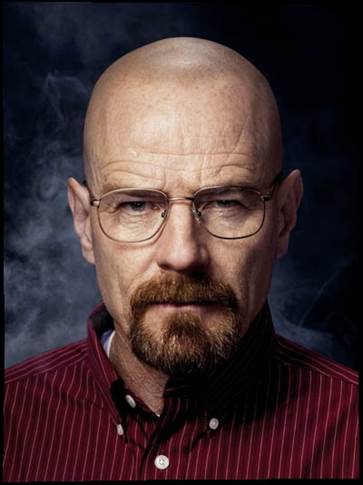
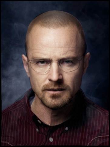
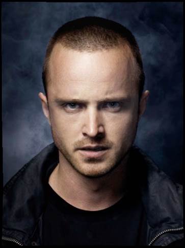
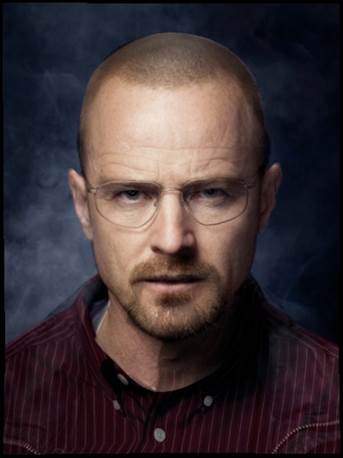
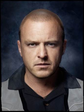
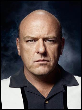
Original Images used:

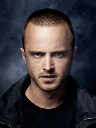
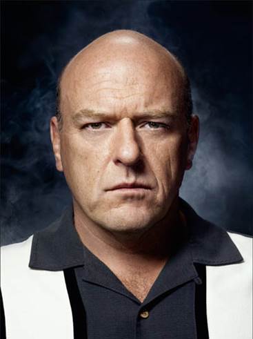
A B C
Images taken from : http://www.amc.com/shows/breaking-bad/extras/breaking-bad-season-4-character-portraits
Copyright AMC Network Entertainment LLC. All rights reserved.